Theorerical background
What is a tesseroid anyway?
A tesseroid, or spherical prism, is segment of a sphere. It is delimited by:
2 meridians, \(\lambda_1\) and \(\lambda_2\)
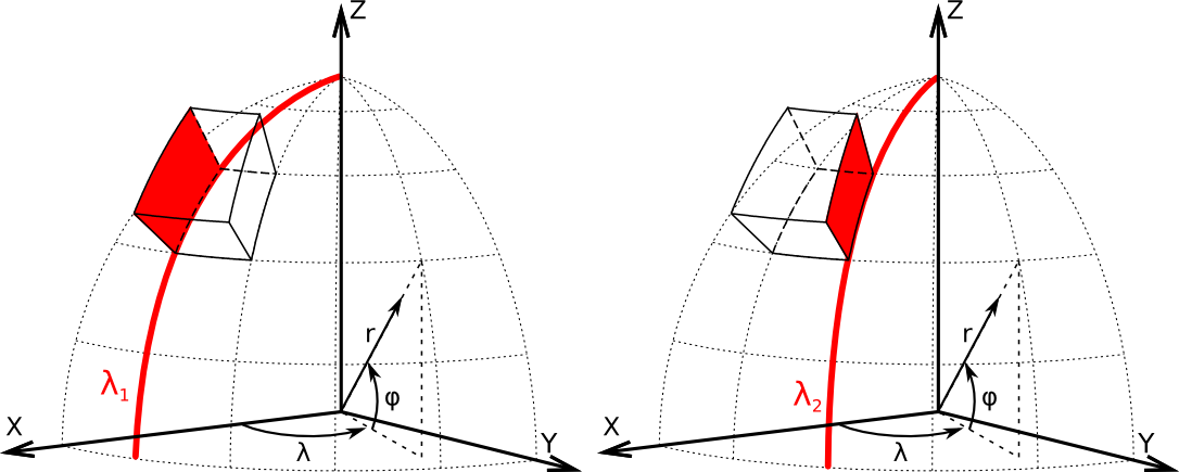
2 parallels, \(\phi_1\) and \(\phi_2\)
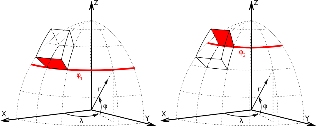
2 spheres of radii \(r_1\) and \(r_2\)
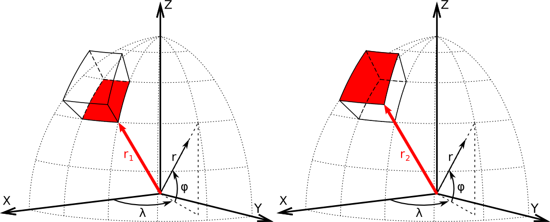
Original images (licensed CC-BY) at doi:10.6084/m9.figshare.1495537.
About coordinate systems
The figure bellow shows a tesseroid, the global coordinate system (X, Y, Z), and the local coordinate system (\(x,\ y,\ z\)) of a point P.
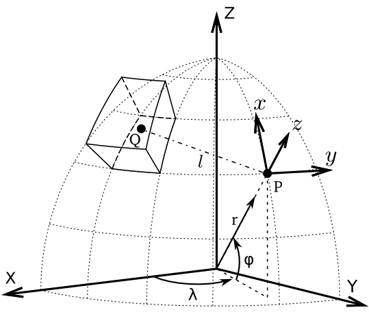
View of a tesseroid, the integration point Q, the global coordinate system (X, Y, Z), the computation P and it’s local coordinate system (\(x,\ y,\ z\)). \(r,\ \phi,\ \lambda\) are the radius, latitude, and longitude, respectively, of point P. Original image (licensed CC-BY) at doi:10.6084/m9.figshare.1495525.
The global system has origin on the center of the Earth and Z axis aligned with the Earth’s mean rotation axis. The X and Y axis are contained on the equatorial parallel with X intercepting the mean Greenwich meridian and Y completing a right-handed system.
The local system has origin on the computation point P. It’s \(z\) axis is oriented along the radial direction and points away from the center of the Earth. The \(x\) and \(y\) axis are contained on a plane normal to the \(z\) axis. \(x\) points North and \(y\) East.
The gravitational attraction and gravity gradient tensor of a tesseroid are calculated with respect to the local coordinate system of the computation point P.
Warning
The \(g_z\) component is an exception to this. In order to conform with the regular convention of z-axis pointing toward the center of the Earth, this component ONLY is calculated with an inverted z axis. This way, gravity anomalies of tesseroids with positive density are positive, not negative.
Gravitational fields of a tesseroid
The gravitational potential of a tesseroid can be calculated using the formula
The gravitational attraction can be calculated using the formula (Grombein et al., 2013):
The gravity gradients can be calculated using the general formula (Grombein et al., 2013):
where \(\rho\) is density, \(\{x, y, z\}\) correspond to the local coordinate system of the computation point P (see the tesseroid figure), \(\delta_{\alpha\beta}\) is the Kronecker delta, and
\(\phi\) is latitude, \(\lambda\) is longitude, and \(r\) is radius.
Note
The gravitational attraction and gravity gradient tensor are calculated with respect to \((x, y, z)\), the local coordinate system of the computation point P.
Numerical integration
The above integrals are solved using the Gauss-Legendre Quadrature rule (Asgharzadeh et al., 2007):
where \(W_i^r\), \(W_j^{\phi}\), and \(W_k^{\lambda}\) are weighting coefficients and \(N^r\), \(N^{\phi}\), and \(N^{\lambda}\) are the number of quadrature nodes (i.e., the order of the quadrature), for the radius, latitude, and longitude, respectively.
Tesseroids implements a modified version the adaptive discretization algorithm of Li et al (2011). This helps guarantee that the numerical integration will achieve a maximum error of 0.1%.
Warning
The integration error may be larger than this if the computation points are closer than 1km of the tesseroids. This effect is more significant in the gravity gradient components.
Gravitational fields of a prism in spherical coordinates
The gravitational potential and its first and second derivatives for the right rectangular prism can be calculated in Cartesian coordinates using the formula of Nagy et al. (2000).
However, several transformations have to made in order to calculate the fields of a prism in a global coordinate system using spherical coordinates (see this figure).
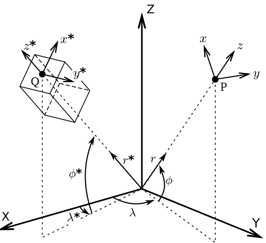
View of a right rectangular prism with its corresponding local coordinate system (\(x^*,\ y^*,\ z^*\)), the global coordinate system (X, Y, Z), the computation P and it’s local coordinate system (\(x,\ y,\ z\)). \(r,\ \phi,\ \lambda\) are the radius, latitude, and longitude, respectively.
The formula of Nagy et al. (2000) require that the computation point be given in the Cartesian coordinates of the prism (\(x^*,\ y^*,\ z^*\) in this figure). Therefore, we must first transform the spherical coordinates (\(r,\ \phi,\ \lambda\)) of the computation point P into \(x^*,\ y^*,\ z^*\). This means that we must convert vector \(\bar{e}\) (from this other figure) to the coordinate system of the prism. We must first obtain vector \(\bar{e}\) in the global Cartesian coordinates (X, Y, Z):
where \(\bar{e}^g\) is the vector \(\bar{e}\) in the global Cartesian coordinates and
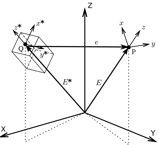
The position vectors involved in the coordinate transformations. \(\bar{E}^*\) is the position vector of point Q in the global coordinate system, \(\bar{E}\) is the position vector of point P in the global coordinate system, and \(\bar{e}\) is the position vector of point P in the local coordinate system of the prism (\(x^*,\ y^*,\ z^*\)).
Next, we transform \(\bar{e}^g\) to the local Cartesian system of the prism by
where \(\bar{\bar{P}}_y\) is a deflection matrix of the y axis, \(\bar{\bar{R}}_y\) and \(\bar{\bar{R}}_z\) are counterclockwise rotation matrices around the y and z axis, respectively (see Wolfram MathWorld).
Which gives us
Note
Nagy et al. (2000) use the z axis pointing down, so we still need to invert the sign of \(z\).
Vector \(\bar{e}\) can then be used with the Nagy et al. (2000) formula. These formula give us the gravitational attraction and the gravity gradient tensor calculated with respect to the coordinate system of the prism (i.e., \(x^*,\ y^*,\ z^*\)). However, we need them in the coordinate system of the observation point P, where they are measured by GOCE and calculated for the tesseroids. We perform these transformations via the global Cartesian system (tip: the rotation matrices are orthogonal). \(\bar{g}^*\) is the gravity vector in the coordinate system of the prism, \(\bar{g}^g\) is the gravity vector in the global coordinate system, and \(\bar{g}\) is the gravity vector in the coordinate system of computation point P.
where
Likewise, transformation for the gravity gradient tensor \(T\) is
Recommended reading
- Smith et al. (2001)
- Wild-Pfeiffer (2008)
References
Asgharzadeh, M. F., R. R. B. von Frese, H. R. Kim, T. E. Leftwich, and J. W. Kim (2007), Spherical prism gravity effects by Gauss-Legendre quadrature integration, Geophysical Journal International, 169(1), 1-11, doi:10.1111/j.1365-246X.2007.03214.x.
Grombein, T.; Seitz, K.; Heck, B. (2013), Optimized formulas for the gravitational field of a tesseroid, Journal of Geodesy, doi: 10.1007/s00190-013-0636-1
Li, Z., T. Hao, Y. Xu, and Y. Xu (2011), An efficient and adaptive approach for modeling gravity effects in spherical coordinates, Journal of Applied Geophysics, 73(3), 221–231, doi:10.1016/j.jappgeo.2011.01.004.
Nagy, D., G. Papp, and J. Benedek (2000), The gravitational potential and its derivatives for the prism, Journal of Geodesy, 74(7-8), 552-560, doi:10.1007/s001900000116.
Nagy, D., G. Papp, and J. Benedek (2002), Corrections to “The gravitational potential and its derivatives for the prism,” Journal of Geodesy, 76(8), 475-475, doi:10.1007/s00190-002-0264-7.
Smith, D. A., D. S. Robertson, and D. G. Milbert (2001), Gravitational attraction of local crustal masses in spherical coordinates, Journal of Geodesy, 74(11-12), 783-795, doi:10.1007/s001900000142.
Wild-Pfeiffer, F. (2008), A comparison of different mass elements for use in gravity gradiometry, Journal of Geodesy, 82(10), 637-653, doi:10.1007/s00190-008-0219-8.