Calculate the gravity gradient tensor from a DEM
This example demonstrates how to calculate the gravity gradient tensor (GGT) due to topographic masses using tesseroids.
To do that we need:
- A DEM file with lon, lat, and height information;
- Assign correct densities to continents and oceans (we’ll be using a little Python for this);
- Convert the DEM information into a tesseroid model;
- Calculate the 6 components of the GGT;
The file dem_brasil.sh is a small shell script
that executes all the above
(we’ll be looking at each step in more detail):
 1 #!/bin/bash
 2
 3 # First, insert the density information into
 4 # the DEM file using the Python script.
 5 python dem_density.py dem.xyz > dem-dens.txt
 6
 7 # Next, use the modified DEM with tessmodgen
 8 # to create a tesseroid model
 9 tessmodgen -s0.166667/0.166667 -z0 -v < dem-dens.txt \
10 > dem-tess.txt
11
12 # Calculate the GGT on a regular grid at 250km
13 # use the -l option to log the processes to files
14 # (usefull to diagnose when things go wrong)
15 # The output is dumped to dem-ggt.txt
16 tessgrd -r-60/-45/-30/-15 -b50/50 -z250e03 | \
17 tessgxx dem-tess.txt -lgxx.log | \
18 tessgxy dem-tess.txt -lgxy.log | \
19 tessgxz dem-tess.txt -lgxz.log | \
20 tessgyy dem-tess.txt -lgyy.log | \
21 tessgyz dem-tess.txt -lgyz.log | \
22 tessgzz dem-tess.txt -lgzz.log -v > dem-ggt.txt
Why Python
Python is a modern programming language that is very easy to learn and extremely productive. We’ll be using it to make our lives a bit easier during this example but it is by no means a necessity. The same thing could have been accomplished with Unix tools and the Generic Mapping Tools (GMT) or other plotting program.
If you have interest in learning Python we recommend the excelent video lectures in the Software Carpentry course. There you will also find lectures on various scientific programming topics. I strongly recommend taking this course to anyone who works with scientific computing.
The DEM file
For this example we’ll use ETOPO1 for our DEM.
The file dem.xyz contains the DEM as a 10’ grid.
Longitude and latitude are in decimal degrees
and heights are in meters.
This is what the DEM file looks like (first few lines):
 1 # This is the DEM file from ETOPO1 with 10' resolution
 2 # points in longitude: 151
 3 # Columns:
 4 #  lon         lat       height(m)
 5 -65.000000 -10.000000    157
 6  -64.833333 -10.000000    168
 7  -64.666667 -10.000000    177
 8  -64.500000 -10.000000    197
 9  -64.333333 -10.000000    144
10  -64.166667 -10.000000    178
Notice that Tesseroids allows you to include
comments in the files by starting a line with #.
This figure
shows the DEM ploted in pseudocolor.
The red rectangle is the area
in which we’ll be calculating the GGT.
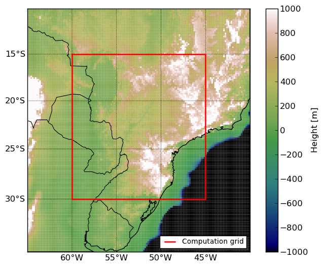
The ETOPO1 10’ DEM of the Parana Basin, southern Brasil.
Assigning densities
Program tessmodgen allows us to provide the density value of each tesseroid through the DEM file. All we have to do is insert an extra column in the DEM file with the density values of the tesseroids that will be put on each point. This way we can have the continents with 2.67 g/cm3 and oceans with 1.67 g/cm3. Notice that the density assigned to the oceans is positive! This is because the DEM in the oceans will have heights bellow our reference (h = 0km) and tessmodgen will automatically invert the sign of the density values if a point is bellow the reference.
We will use the Python script dem_density.py
to insert the density values into our DEM
and save the result to dem-dens.txt:
3 # First, insert the density information into
4 # the DEM file using the Python script.
5 python dem_density.py dem.xyz > dem-dens.txt
If you don’t know Python,
you can easily do this step in any other language
or even in Excel.
This is what the dem_density.py script looks like:
 1 """
 2 Assign density values for the DEM points.
 3 """
 4 import sys
 5 import numpy
 6
 7 lons, lats, heights = numpy.loadtxt(sys.argv[1], unpack=True)
 8
 9 for i in xrange(len(heights)):
10     if heights[i] >=0:
11         print "%lf %lf %lf %lf" % (lons[i], lats[i], heights[i], 2670.0)
12     else:
13         print "%lf %lf %lf %lf" % (lons[i], lats[i], heights[i], 1670.0)
The result is a DEM file with a forth column containing the density values (see this figure):
 1 -65.000000 -10.000000 157.000000 2670.000000
 2 -64.833333 -10.000000 168.000000 2670.000000
 3 -64.666667 -10.000000 177.000000 2670.000000
 4 -64.500000 -10.000000 197.000000 2670.000000
 5 -64.333333 -10.000000 144.000000 2670.000000
 6 -64.166667 -10.000000 178.000000 2670.000000
 7 -64.000000 -10.000000 166.000000 2670.000000
 8 -63.833333 -10.000000 164.000000 2670.000000
 9 -63.666667 -10.000000 189.000000 2670.000000
10 -63.500000 -10.000000 210.000000 2670.000000
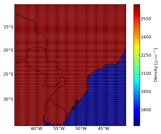
Density values. 2.67 g/cm3 in continents and 1.67 g/cm3 in the oceans.
Making the tesseroid model
Next, we’ll use our new file dem-dens.txt
and program tessmodgen to create
a tesseroid model of the DEM:
 7 # Next, use the modified DEM with tessmodgen
 8 # to create a tesseroid model
 9 tessmodgen -s0.166667/0.166667 -z0 -v < dem-dens.txt \
10 > dem-tess.txt
tessmodgen places a tesseroid on each point of the DEM.
The bottom of the tesseroid is placed on a reference level
and the top on the DEM.
If the height of the point is bellow the reference,
the top and bottom will be inverted
so that the tesseroid isn’t upside-down.
In this case,
the density value of the point
will also have its sign changed
so that you get the right density values
if modeling things like the Moho.
For topographic masses,
the reference surface is h = 0km (argument -z).
The argument -s is used
to specify the grid spacing (10’)
which will be used to set
the horizontal dimensions of the tesseroid.
Since we didn’t pass the -d argument
with the density of the tesseroids,
tessmodgen will expect a fourth column
in the input with the density values.
The result is a tesseroid model file that should look somthing like this:
 1 # Tesseroid model generated by tessmodgen 1.1dev:
 2 #   local time: Wed May  9 19:08:12 2012
 3 #   grid spacing: 0.166667 deg lon / 0.166667 deg lat
 4 #   reference level (depth): 0
 5 #   density: read from input
 6 -65.0833335 -64.9166665 -10.0833335 -9.9166665 157 0 2670
 7 -64.9166665 -64.7499995 -10.0833335 -9.9166665 168 0 2670
 8 -64.7500005 -64.5833335 -10.0833335 -9.9166665 177 0 2670
 9 -64.5833335 -64.4166665 -10.0833335 -9.9166665 197 0 2670
10 -64.4166665 -64.2499995 -10.0833335 -9.9166665 144 0 2670
and for the points in the ocean (negative height):
9065 -40.0833335 -39.9166665 -19.9166665 -19.7499995 0 -19 -1670
Calculating the GGT
Tesseroids allows use of custom computation grids
by reading the computation points from standard input.
This way,
if you have a file with lon, lat, and height coordinates
and wish to calculate any gravitational field in those points,
all you have to do is redirect stardard input to that file
(using <).
All tess* programs will calculate their respective field,
append a column with the result to the input
and print it to stdout.
So you can pass grid files
with more than three columns,
as long as the first three
correspond to lon, lat and height.
This means that you can pipe the results
from one tessg to the other
and have an output file with many columns,
each corresponding to a gravitational field.
The main advantage of this approach is that,
in most shell environments,
the computation of pipes is done in parallel.
So, if your system has more than one core,
you can get parallel computation of GGT components
with no extra effort.
For convience, we added the program tessgrd to the set of tools, which creates regular grids and print them to standard output. So if you don’t want to compute on a custom grid (like us), you can simply pipe the output of tessgrd to the tess* programs:
12 # Calculate the GGT on a regular grid at 250km
13 # use the -l option to log the processes to files
14 # (usefull to diagnose when things go wrong)
15 # The output is dumped to dem-ggt.txt
16 tessgrd -r-60/-45/-30/-15 -b50/50 -z250e03 | \
17 tessgxx dem-tess.txt -lgxx.log | \
18 tessgxy dem-tess.txt -lgxy.log | \
19 tessgxz dem-tess.txt -lgxz.log | \
20 tessgyy dem-tess.txt -lgyy.log | \
21 tessgyz dem-tess.txt -lgyz.log | \
22 tessgzz dem-tess.txt -lgzz.log -v > dem-ggt.txt
The end result of this is file dem-ggt.txt,
which will have 9 columns in total.
The first three are the lon, lat and height coordinates
generated by tessgrd.
The next six will correspond to each component
of the GGT calculated by tessgxx, tessgxy, etc., respectively.
The resulting GGT is shown in this figure.
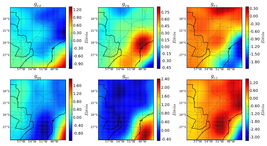
GGT of caused by the topographic masses.
Making the plots
The plots were generated using
the powerfull Python library Matplotlib.
The script plots.py is somewhat more complicated than dem_density.py
and requires a bit of “Python Fu”.
The examples in the Matplotlib website
should give some insight into how it works.
To hanble the map projections,
we used the Basemap toolkit of Matplotlib.